In this blog post I will explain how you can automatise the creation of R-Markdown documents.

My main motivation for this was that I had a document where I had to create an R Markdown with several very similar sections. Of course I could write each section with new code, but I do not like repetive tasks (they are boring and tiring), so I decided to automatise the creation of sections, tables and graphs.

I do not want to run all the (quite long) data creation process when building the R-Markdown. So firstly I created a script to create the data and saved it with RDS format (I am also a big fan of fst format, but the data was in a nested list, which cannot be saved in fst-Format).

When creating the R-Markdown the data was ready to use.

The next step was to create the introduction of the document. I wanted to put all the creation of the outputs into functions.

Libraries loading

First thing is to load some of the necessary libraries

library(DT)
library(data.table)
library(knitr)
library(ggplot2)
suppressPackageStartupMessages(library(plotly))
knitr::opts_chunk$set(echo = TRUE)

Results: asis

So my way to go was to use the option results = "asis" in the setting of R-Markdown:

```{r asis_example, results = "asis"}
cat(paste0("- `", names(iris), "`"), sep = "\n")
```

This option tells knitr not to wrap your text output in verbatim code blocks, but treat it “as is.”

Output:

cat(paste0("- ", names(iris)), sep = "\n\n")

Sepal.Length
Sepal.Width
Petal.Length
Petal.Width
Species

Usage of cat

It is important (and a bit laborious) to wrap outputs into cat, otherwise it is not treated correctly by R-Markdown. Moreover \n\n is used to start a new line. Here a bad example:

Output:

print(paste0("- ", names(iris), "\n\n"))

[1] “- Sepal.Length” “- Sepal.Width” “- Petal.Length” [4] “- Petal.Width” “- Species”

Usage of echo

It is important to set the option echo = FALSE, otherwise the input code is also printed out. Some introduction with header could look like this:

```{r intro, echo = FALSE, results = "asis"}
      cat("# General Information  {-}\n")
      cat("**Model creator:**\n\n")
      cat("Philipp Probst")
      cat("\n\n")
      cat("**Creation Date of Models:**\n\n")
      knitr::knit_print(as.Date(Sys.Date()))
```

Output:

General Information

Model creator:

Philipp Probst

Creation Date of Models:

[1] “2024-01-12”

As you can see in the above code I used rknitr::knit_print` to have a proper output for the date. This will be necessary in many cases (e.g. also when printing tables or plots).

Tabs

Moreover to show things by using the space ideally and in a nice way is to use tabs.

For this we have to add \{.tabset \} behind the header. \{.unnumbered \} can be used to set off numbering of the header, if in general it is turned on (e.g. in the preamble: number_sections: true).

```{r tabs, echo = FALSE, results = "asis"}
cat("## My Tabs header {.tabset .unnumbered} \n\n")
cat(paste0("### ", "Tab 1", " {.unnumbered} \n\n"))
cat("ABC \n\n")
cat("### Tab 2  {-}\n\n")
cat("DEF \n\n")
cat("## New Section\n\n")
```

Output:

My Tabs header

Tab 1

ABC

Tab 2

DEF

New Section

Folding

Another nice tool is that you can fold some section, text, graphs, etc.

For this you have to use the HTML <details> tag:

```{r folds, echo = FALSE, results = "asis"}
cat("Some text\n\n")
cat("<details>\n\n")
cat("<summary>Hidden Text</summary>\n\n")
cat("DEF \n\n")
cat("</details>\n\n")
```

Output:

Some text

Hidden Text

DEF

Printing tables and plots

Tables

For printing tables it is necessary to wrap the function knitr::knit_print() and DT::datatable around them. Then it has also nice sorting abilities.

It is also possible to print a table by using print(kable(…)) although it does not have the nice abilities of DT::datatable .

```{r tables, echo = FALSE, results = "asis"}
knitr::knit_print(DT::datatable(iris[1:6,]))
print(kable(iris[1:6,]))
```

Output:

Sepal.Length	Sepal.Width	Petal.Length	Petal.Width	Species
5.1	3.5	1.4	0.2	setosa
4.9	3.0	1.4	0.2	setosa
4.7	3.2	1.3	0.2	setosa
4.6	3.1	1.5	0.2	setosa
5.0	3.6	1.4	0.2	setosa
5.4	3.9	1.7	0.4	setosa

Plots

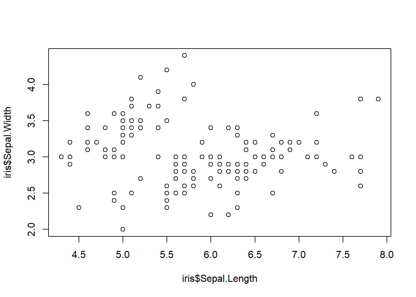
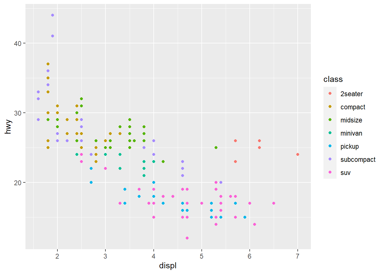
Base-R, ggplot2 or plotly plots do not need any adjustment in the results = "asis" mode.

```{r plots, echo = FALSE, results = "asis"}
plot(iris$Sepal.Length, iris$Sepal.Width)
ggplot(mpg, aes(displ, hwy, colour = class)) + geom_point()
plot_ly(data = iris, x = ~Sepal.Length, y = ~Petal.Length)
```

Output:

::: {.cell-output-display}

:::

I will add more tricks in the next blog post.

E.g. it will include the following

Functions that automatically create tabs
How to chunkify